

Measures of Dispersion
Describing a dataset’s center using only a measure of location, such as the mean or median, is rarely sufficient. It is for this reason that measures of location are paired with measures of dispersion. Unlike measures of location which describe the typical location of a dataset, measures of dispersion describe a dataset’s spread. Here, two of the most common measures of dispersion—the range (R) and the standard deviation (s)—as well as a third, the average moving range (mR), will be discussed.
Although the average moving range is an often overlooked measure of dispersion, it is included in this discussion for the role it plays in the construction of an XmR chart. Without the average moving range, the calculation of process limits for a dataset composed of logically comparable individual values would not exist.
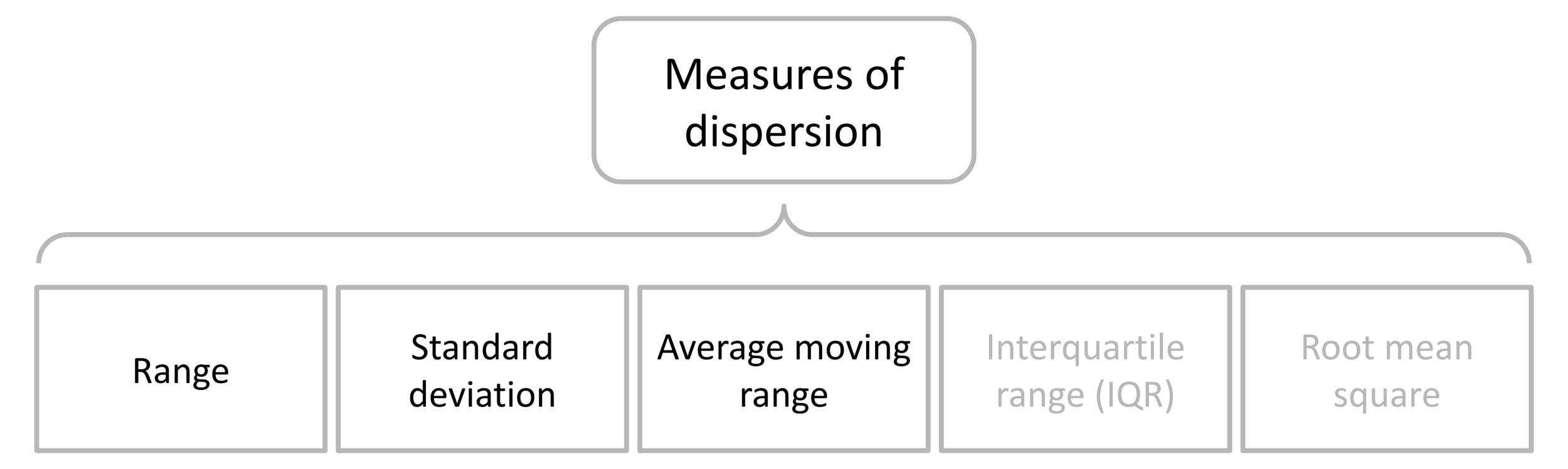
Figure 1. Common measures of dispersion.
Table of contents
Range
The simplest measure of dispersion to calculate and understand is the range. To calculate it, subtract the smallest value in a dataset from the largest value. The value that results from this calculation describes the datasets spread, the extent to which the values are dispersed.

The range’s simplicity is both a strength and a weakness. While the simplicity makes it easy to calculate it also makes it susceptible to extreme or dissimilar values. This makes the range a less accurate measure of dispersion than the standard deviation, especially when dealing with large datasets.
As was the case with measures of location, the measure of dispersion you use should be driven by your analytical goals. The range can be a satisfactory measure of dispersion assuming its limitations are understood.
The maximum, minimum, and range for the 12 annual salaries shown in Table 1 are $450,000, $43,000, and $407,000 respectively. Given these values, does the range provide an accurate measure of dispersion for the dataset?
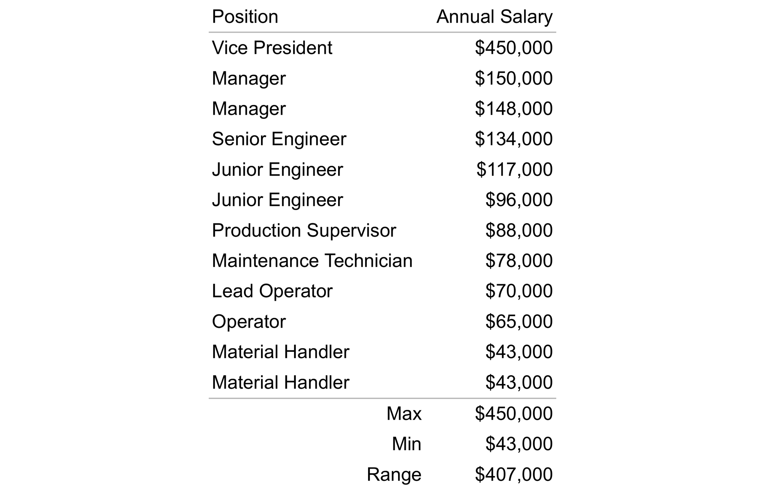
Table 1. Annual salaries for 12 employees with the associated max, min, and range.
Assuming your goal is a simple understanding of the salary spread, using the range as a measure of dispersion may be satisfactory. However, if you’re looking for a measure of dispersion that is analytically more nuanced, the standard deviation is likely the better choice.
Standard deviation
Denoted as s, the standard deviation incorporates all of the values in a dataset into its calculation and measures how far those values deviate from the mean. This makes the standard deviation a more practical measure of dispersion than the range.
The standard deviation is calculated using the following formula:

Here, s is the standard deviation, √ is the square root, Xi is the i-th value in the dataset, X is the mean, n is the number of values in the dataset, and ∑(Xi-X)2 is the sum of the squared deviations of the individual values from the mean.
The sample standard deviation (s) should not be confused with the population standard deviation, denoted by sigma (𝜎). While the sample standard deviation is calculated from a subset of data taken from a larger population and uses n - 1 as the denominator, the population standard deviation is calculated from the entire population and uses n as the denominator.
In practice, the standard deviation is calculated in six steps:
Calculate the mean of the dataset (X).
Find the deviation of each value from the mean (Xi − X).
Square each deviation obtained in step 2.
Sum all of the squared deviations.
Divide the sum by n − 1, where n is the number of values in the dataset.
Take the square root of the result from step 5. This value is the standard deviation.
Although it is more complicated to calculate than the range, its intricacies make it a more robust measure of dispersion.
Table 2 shows the 12 annual salaries from Table 1 and the associated standard deviation of $109,290.69. Recall that the range for the same dataset was $407,000.
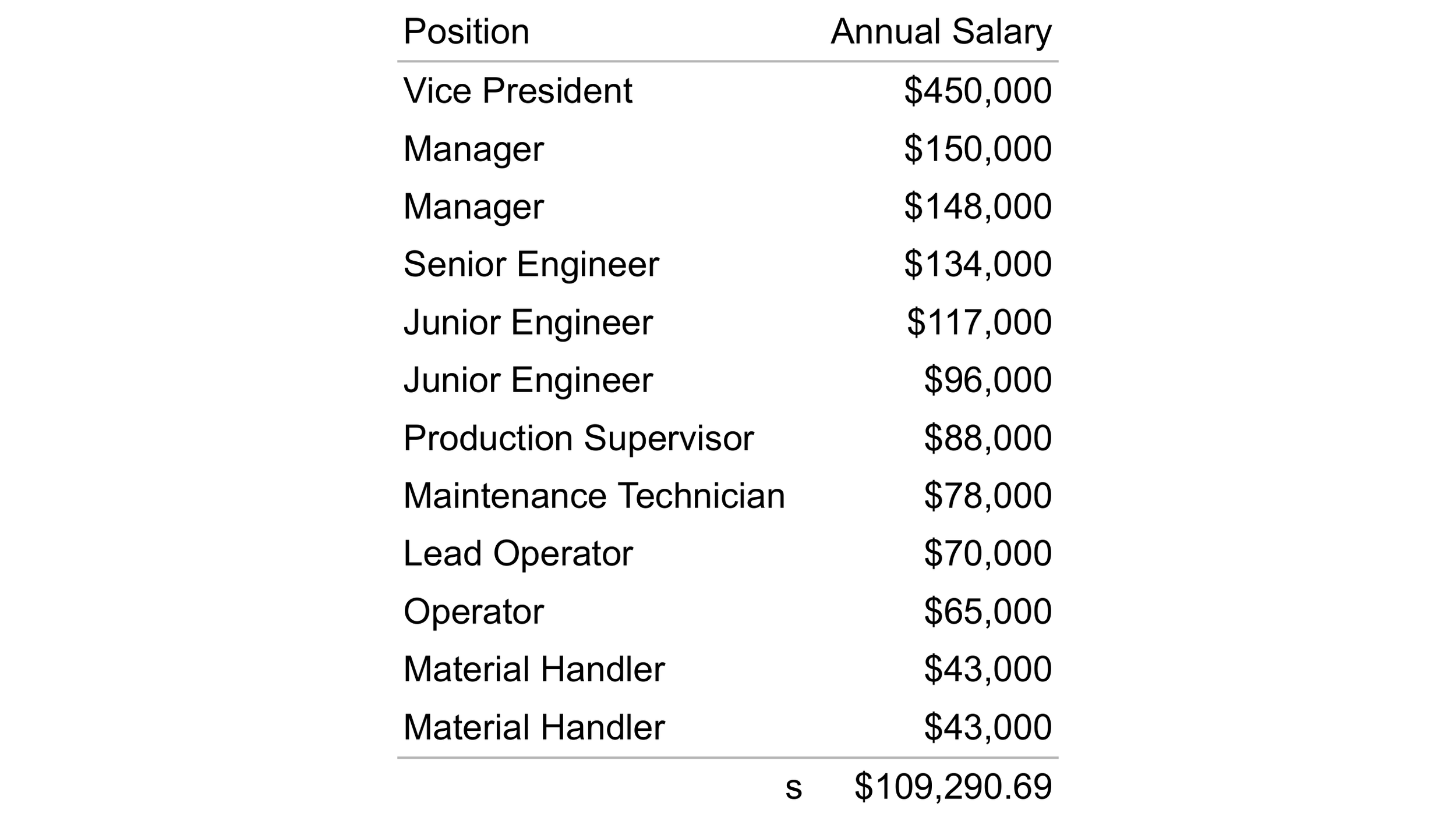
Table 2. Annual salaries for 12 employees with the associated median.
With the dataset already in descending order, the first step in calculating the median is complete. The second step is to determine the middle value of the ordered list. The dataset contains 12 salaries. Therefore, n = 12 and the even case of the piecewise function for calculating the median applies as follows:
Average moving range
When a dataset is composed of logically comparable individual values with a time-order sequence, the value-to-value difference is summarized by the average moving range. When a dataset does not have a time ordered sequence, any efforts to calculate the average moving range will be erroneous, although a pseudo-average moving range can be calculated from a dataset with a completely random sequence.
The average moving range plays a critical role in the calculation of the process limits for an XmR chart and is included here for that reason.
Calculating the average moving range first requires the calculation of the moving range. The moving range is the absolute value of the difference between successive values in a dataset. Thus, it is calculated using the formula:

Here, mRi is the moving range for the i-th pair of successive values; Xi is the current value, and Xi-1 is the previous value. The vertical bars (||) indicate the absolute value.
As an example, take the 12 diameters from a manufacturing process shown in Table 3.
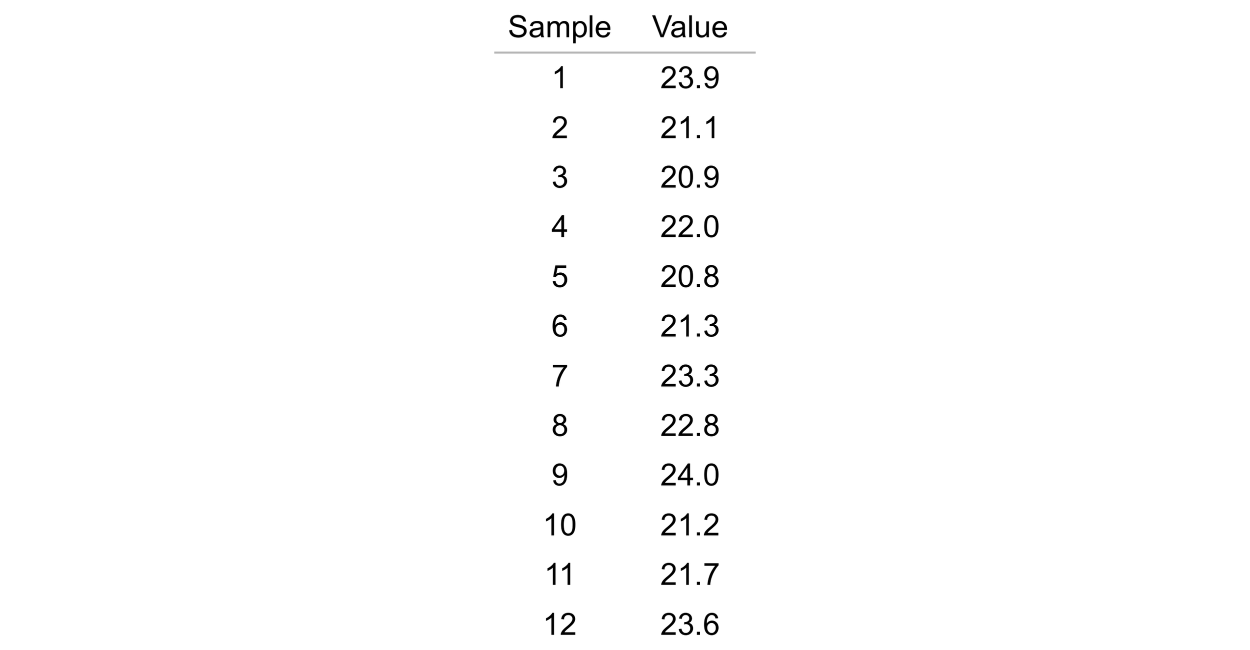
Table 3. Manufacturing process diameter measurements.
The first value in Table 3 is 23.9 units and the second value is 21.1 units. The absolute value of the difference between 23.9 and 21.1 yields a moving range of 2.8 units.

The second value in Table 3 is 21.1 units and the third value is 20.9 units. This makes the second moving range 0.2 units.

Repeating this process of calculating the absolute value of the difference between successive values yields the moving range shown in Table 4.
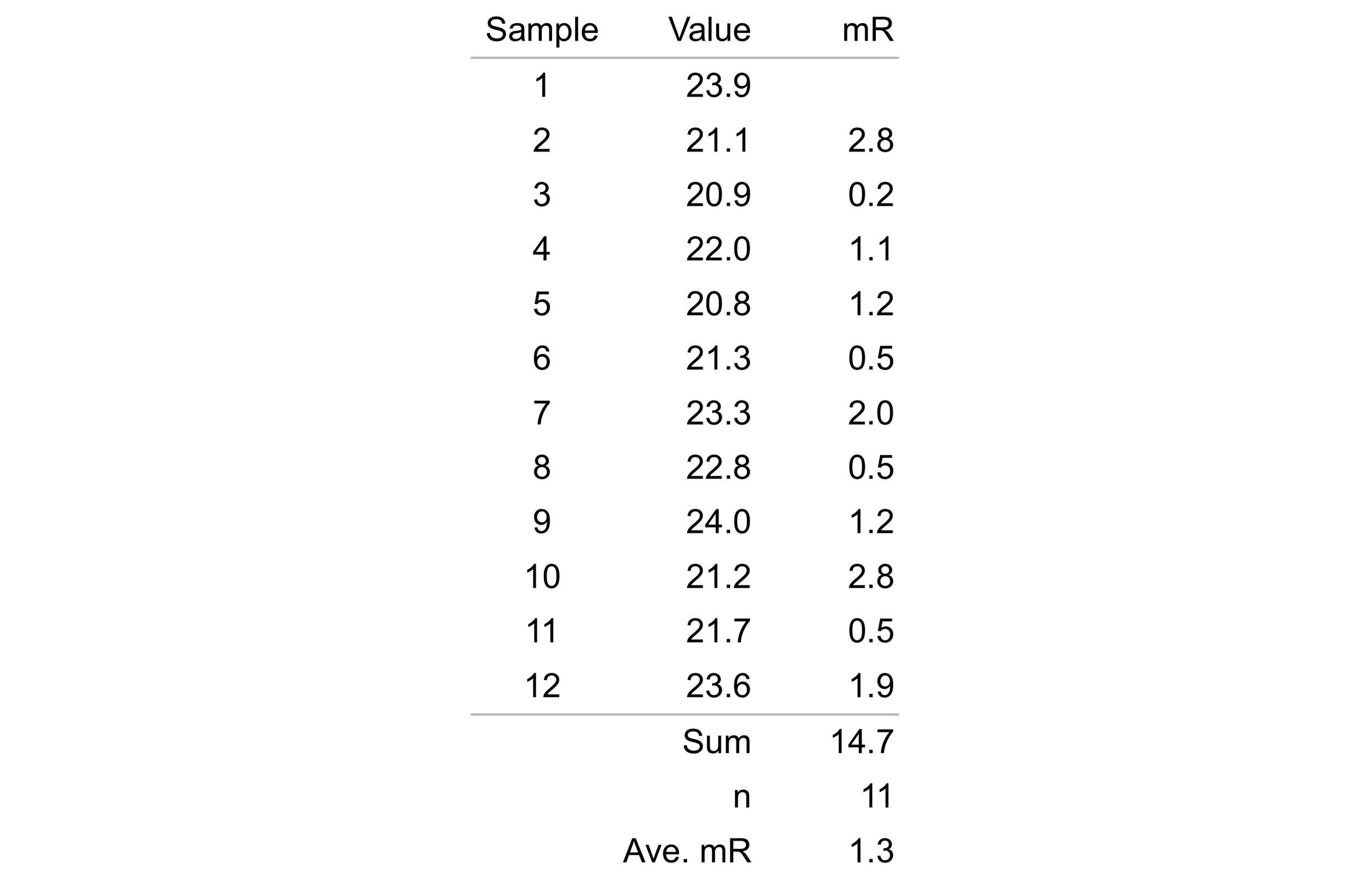
Table 4. Manufacturing process diameter measurements with associated moving ranges.
With the moving ranges in hand, calculating the average moving range is trivial. It is the average of the moving ranges and is described by the formula:

Here, the sum of the moving ranges (14.7) is divided by the number of moving ranges (11). Thus, the average moving range for the moving ranges in Table 4 is 1.3 units.
