

The challenge of manufacturing
For as long as humans have been making things, efforts have been made to make things that are the same. This seemingly simple task, while easy to state, is anything but when put into practice. Producing multiples of the same part, assembly, or product that are functionally identical is more complicated than it first appears. Measurements of multiples quickly reveal that no two things produced by the same process will ever be the same (the process principle). Differences in outputs are an intrinsic and defining feature of all processes. Thus, the challenge of manufacturing is the challenge of understanding and mitigating differences. The extent to which the sequential outputs of a process or system differ is called variation.
It is easy to manufacture one of something because one of something is self-contained. Outside of engineering drawings, there are no analogues for comparing individually produced parts. While measurements of manufactured product reveals how said product conforms or deviates to drawings, individual measurements make no statements and answer no questions about the underlying production process. They reveal nothing about how a manufacturing process has behaved in the past or how it will behave in the future. To do that, the same process must be used to manufacture multiples. Then, and only then, can measurements of those multiples be compared and a picture of the underlying causal system be painted.
Having produced multiples of the same part, it is guaranteed that measurements will reveal differences, though it is hoped that these differences will be negligible. But just as no two snowflakes are alike, no two parts produced by the same process will ever be identical. Variation, whether we recognize it or not, always asserts its influence.
Making sense of the variation that emerges from measuring the outputs of a process has historically fallen to the task of specification limits or “spec” limits. These limits define how large or small a dimensional measurement or performance characteristic can be before it is deemed unacceptable by the customer. This is epitomized by the rectangular loss function shown in Figure 1. The sharp cutoffs at the Lower Specification Limit (LSL) and Upper Specification Limit (USL) imply that all values within these limits are “good”, while everything outside is considered “bad” and must be either reworked or scrapped.
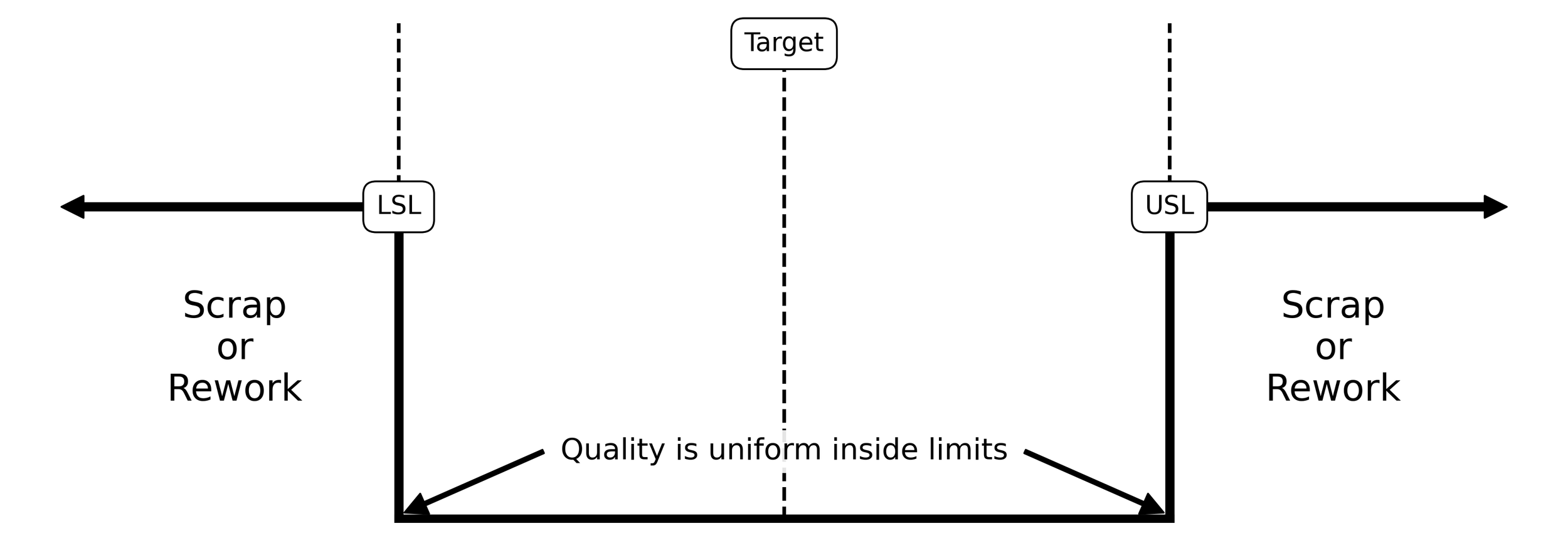
Figure 1. Square loss function and specification limits or “spec” limits impart a binary view.
This binary concept of variation, while novel for its time, complicated the task of making things. Rather than work toward an idealized process of fabricate, pack, and ship, a series of steps that sorted good parts from bad parts became the norm (see Figure 2). This sorting process has become the hallmark of manufacturing known as inspection.
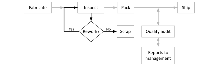
Figure 2. The engineering concept of specifications imparts complexity into the process of manufacturing in the form of inspection.
Since its inception, inspection has obscured the intent of manufacturing from its more fundamental purpose. That purpose is not to produce parts within spec. It is to produce parts that are functionally identical. This is achieved when manufacturing efforts aim to produce parts that are on-target with minimum variance. This operational definition—introduced by Dr. Genichi Taguchi in September of 1960—is how world-class quality is achieved. It deems the binary view of manufacturing imparted by spec limits as unacceptable and replaces it with an endless cycle of continual improvement. This is epitomized by the quadratic loss function of the form:

Here, L(x) is the loss function, K is a numeric constant (often expressed in terms of dollars per measurement unit squared), x is the value for a performance or quality characteristic, T is the target value for the performance or quality characteristic, and (x - T)^2 is the squared deviation of the performance or quality characteristic from the target.
When visualized as a parabola, the quadratic loss function takes the form shown in Figure 3.
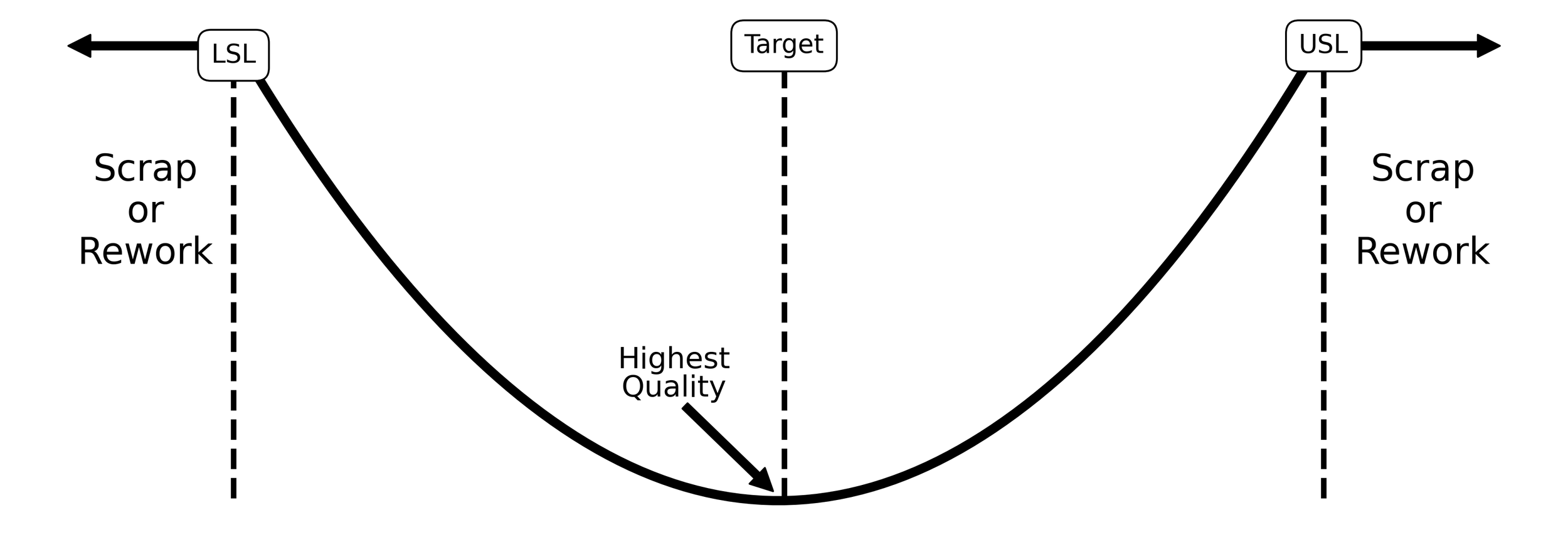
Figure 3. The Taguchi concept of loss due to poor quality is governed by a quadratic loss function within some region close to the target.
The vertex of the parabola, centered at the target, is where a process will produce the highest quality. The further a quality or performance characteristic diverges from this nominal, the larger the loss due to poor quality. This loss increases quadratically until the loss function reaches the specification limits. When a performance or quality characteristic reaches the spec limits, the maximum loss due to poor quality is incurred. In instances where rework can be performed, a portion of the loss is recovered. In instances where parts must be scrapped, the full loss due to poor quality is realized.
The Taguchi loss function, although not perfect, is a more realistic model of loss due to poor quality. Where loss under the square loss function in Figure 1 occurs abruptly, loss under the Taguchi loss function is incremental. This incremental loss encourages activities that aim to manufacture product that is virtually identical.
The thought of producing virtually identical product may seem farcical, yet, the likelihood of realizing this goal increases when we understand variation. Understanding variation allows us to discriminate between signals and noise. It allows us to determine when it is economical to take actions to improve a process and when it is economical to leave a process alone. But this is only possible when we have tool capable of the task. That tool, as you will come to see, is the process behavior chart (otherwise known as a control chart).
“Planning requires prediction.”
— W. Edwards Deming, Out of the Crisis
Shewhart & the two types of variation
In the mid-1920s, the physicist Walter Shewhart established the framework for understanding variation that is as effective today as it was then. While working at Bell Labs, Shewhart came to understand that variation is a relentless force influencing all manufacturing processes. It was from this understanding that Shewhart established that, as summarized by Donald J. Wheeler on page 4 of Understanding Statistical Process Control,
“While every process displays variation, some processes display controlled variation, while other processes display uncontrolled variation.”
This distinction between controlled variation and uncontrolled variation is the core insight of Shewhart’s work at Bell Labs. It is from this finding that our understanding of variation emerged and with it the development of the only tool capable of discriminating between the two types of variation—the process behavior chart.
The first type of variation, common causes of routine variation, is an innate and natural feature of all processes. When influenced by only common causes, a process displays a consistent pattern of variation over time. An idealized example of this concept is shown in Figure 4. Here, the quality characteristic for a series of discrete parts produced by the same process on different days is shown. The consistency of the distributions from day-to-day regarding its shape, center, and spread, indicates that only common causes of routine variation influence process behavior. These differences are the product of the to-be-expected variation that is an unavoidable feature of making things.
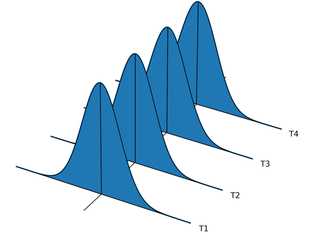
Figure 4. When a process is influenced by only common causes of routine variation it
Assignable causes of exceptional variation, on the other hand, are an extrinsic and unexpected feature of process behavior. Processes influenced by assignable causes display patterns of variation that are inconsistent over time. An idealized example of this concept is shown in Figure 5. Here, the quality characteristic for a series of discrete parts produced by the same process on different days is shown. The inconsistency of the distribution from day-to-day regarding its shape, center, and spread, the way it erratically shifts, expands, and contracts, indicates that differences between parts are the product of both common causes of routine variation and assignable causes of exceptional variation. Although assignable causes are few in number they are dominant in their effect. Thus, the presence of assignable causes ensures future process behavior cannot be predicted (within limits).
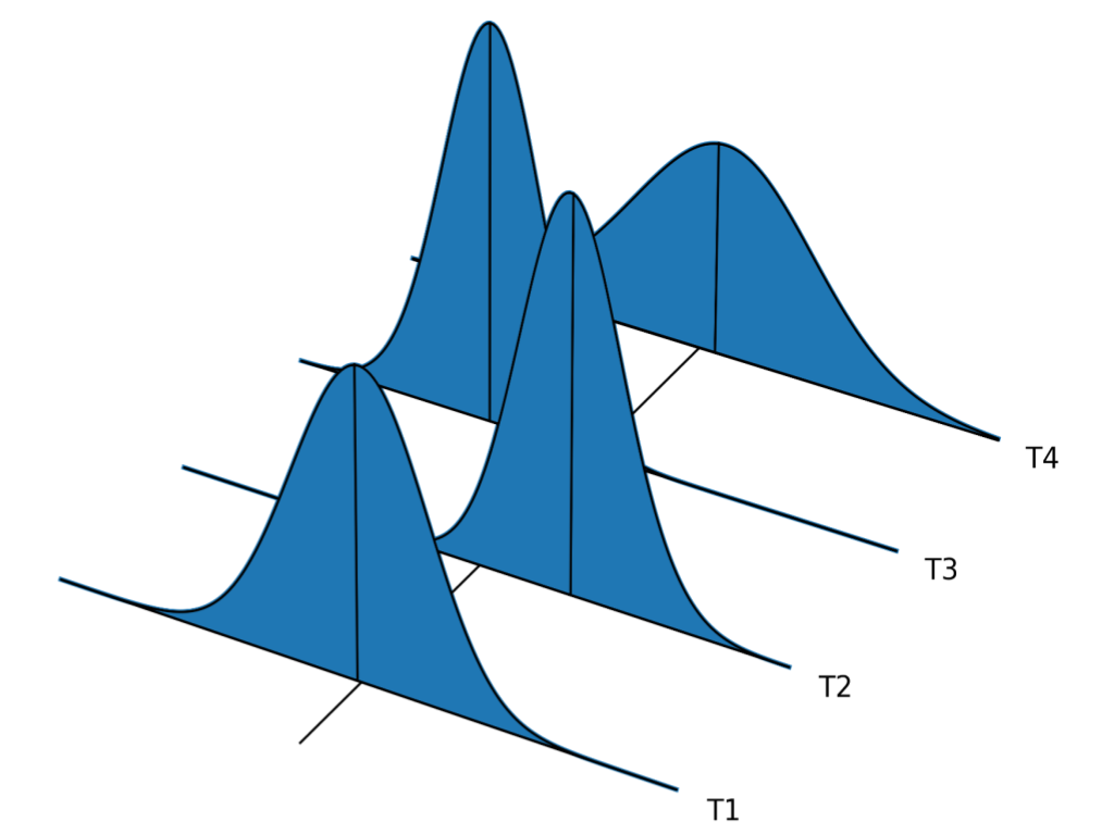
Figure 5. Idealized concept of a process influenced by assignable causes of exceptional variation.
Since, at its core, management is prediction, the influence of assignable causes of exceptional variation on process behavior makes the job of management impossible. It reduces it to gut feelings and guesswork. While even a broken clock is right twice a day, the improvement of quality and reduction of costs requires a more robust, repeatable, and formal strategy. Recognizing this, and having established the distinction between the two types of variation, Shewhart got to work building a tool capable of discriminating between them. The result was the process behavior chart—what Shewhart called a control chart.