Capability Clarity
The only time the process capability indices make practical sense (that is to say they are well-defined and useful) is when a process has been shown to be operating in a state of statistical control. This is the state that is achieved when, by using a process behavior chart, future process behavior can be predicted within limits i.e. the process is characterized as predictable. This occurs when all of the values on a process behavior chart fall within the process limits. Without this knowledge, the process capability indices may be misleading or altogether false indicators of what the process will do in the future.
The logic for using the process capability indices is outlined in the flowchart shown in Figure 1. Here, efforts always begin with characterization (to learn more about characterization click here). When a process is characterized as predictable, the logic on the left side of the flowchart is followed. In these instances, the underlying causal system is influenced by only common causes of routine variation. While many in number, common causes are minimal in their effect. Thus, a predictable process will change very little over time. Observations collected from a predictable process can be used to compute summary statistics that both describe properties of the data and estimate process parameters (like the process capability indices).
When a process is characterized as unpredictable, the logic on the right side of the flowchart is followed. In these instances, the underlying causal system is influenced by both common causes of routine variation and assignable causes of exceptional variation. While few in number, assignable causes are dominant in their effect. Thus, the underlying causal system will bounce and shift in unpredictable ways. Observations collected from an unpredictable process can be used to compute summary statistics but those summary statistics ONLY describe properties of the data. Attempts to use these statistics to estimate process parameters (like the process capability indices) are functionally meaningless because the underlying causal system is always changing. The only time process parameters are well-defined is when a process is operated predictably.
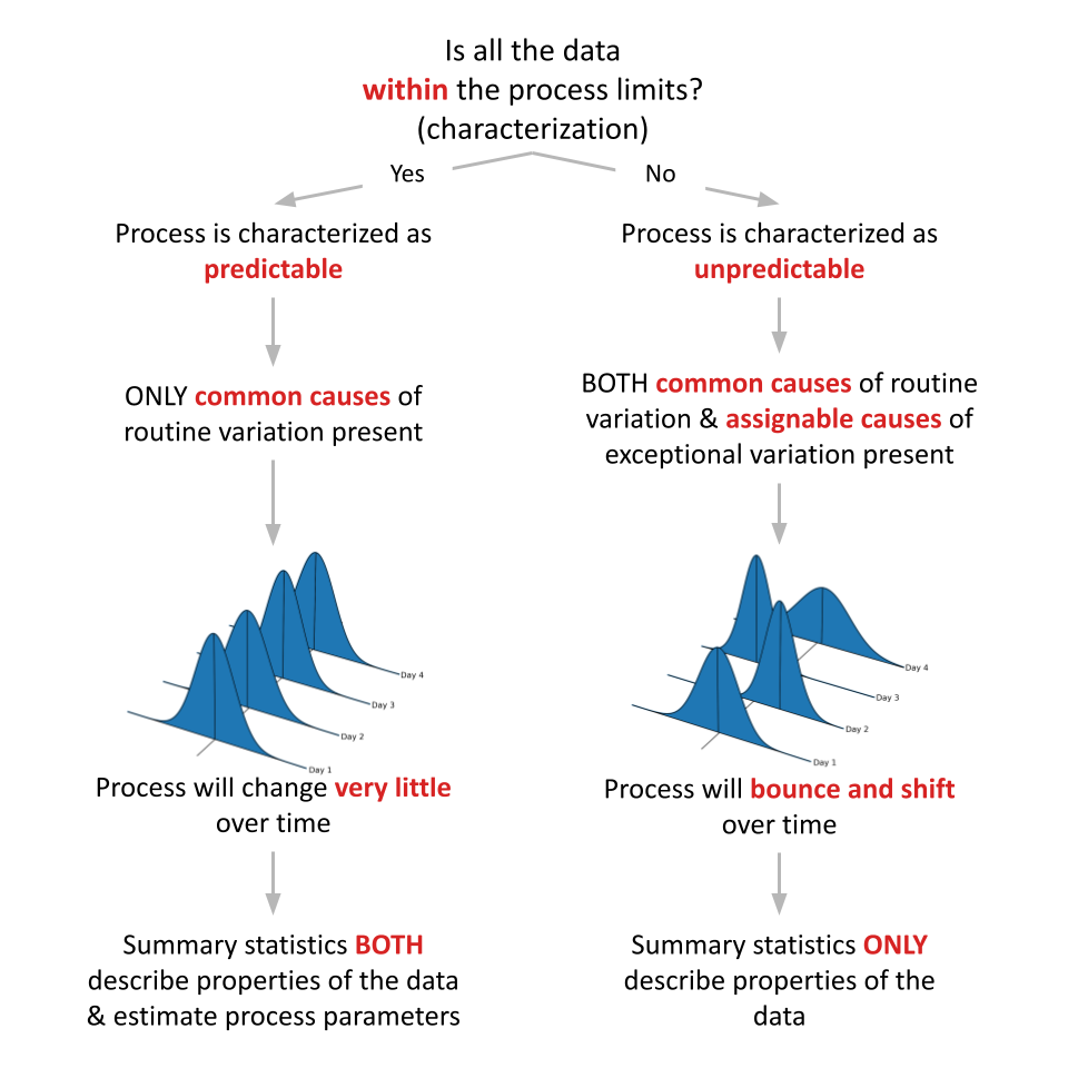
Figure 1. Flowchart outlining the logic for when the process capability indices are reliable.
Although you may be required to report the process capability indices regardless of the characterization, the knowledge revealed by characterization is quintessential to how you move forward. When a process is operated unpredictably, any changes to the process that do not address the influence of assignable causes will be worthless. While few in number, assignable causes are dominant in their effect. The only way to improve an unpredictable process is to eliminate the influence of the assignable causes. The only way to eliminate the influence of assignable causes is to identify them with a process behavior chart. Thus, when required to report the process capability indices, always present them with the associated process behavior chart. This will give the indices visual context that is overlooked when the only the values of the indices are reported.
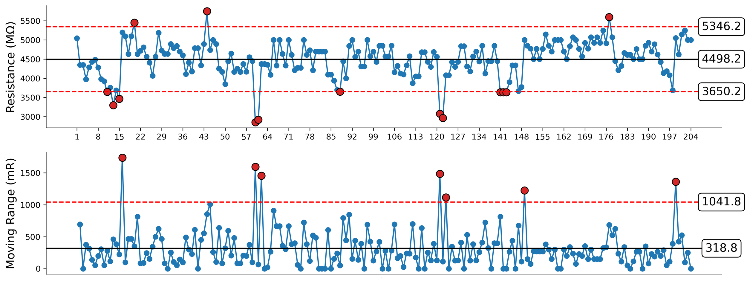
Figure 2. XmR chart of process data.
While process behavior charts reveal the types of variation that influence process behavior, they do not reveal how the process is operating with regard to the specification limits. Thus, in addition to a process behavior chart, process capability indices should also be presented with a capability histogram like the one shown in Figure 3. Capability histograms reveal the shape, center, and spread of process data in the context of the Upper Specification Limit (USL), the Lower Specification Limit (LSL), the target, and the mean of the distribution. The specification limits define the voice of the customer. They define what a customer is willing to pay for and what they will reject.
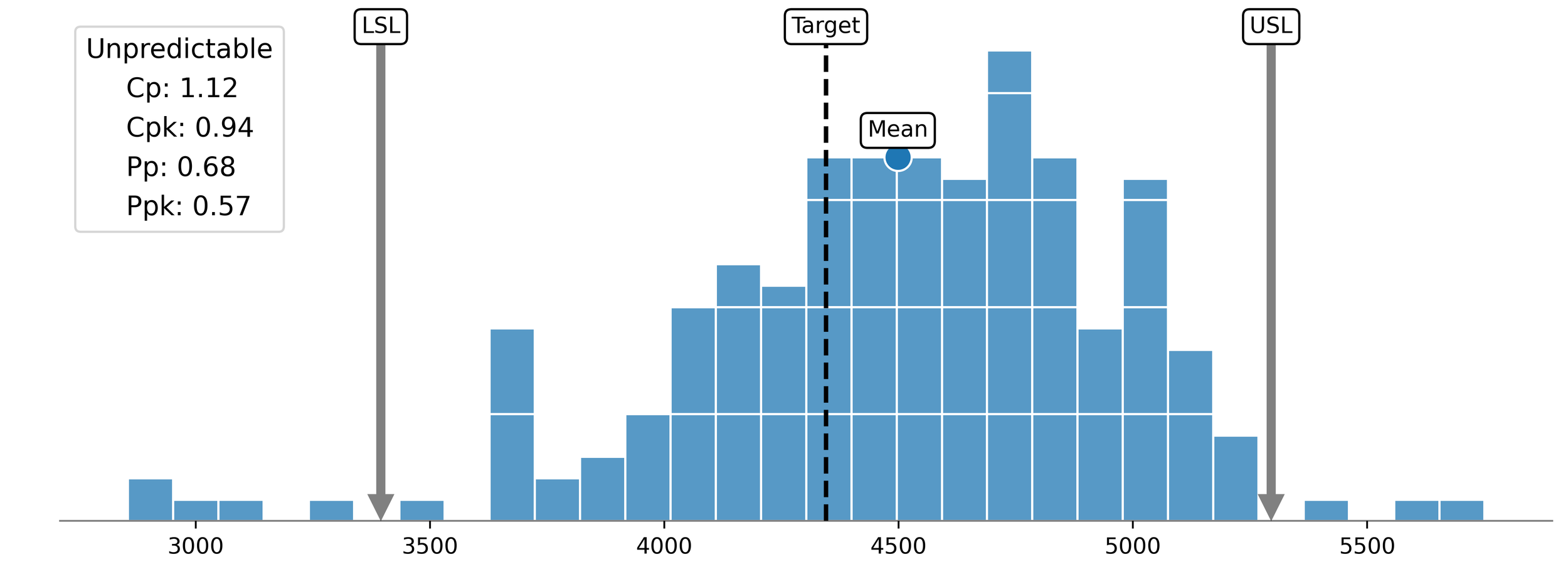
Figure 3. Capability histogram, the associated process capability indices, and the characterization of the underlying causal system.
By presenting the process capability indices with the context of both a process behavior chart and a capability histogram when reporting, a complete picture of the process lifecycle is revealed. The process behavior chart reveals the voice of the process. The capability histogram reveals the voice of the customer. The process capability indices reveal the relationship between the voice of the process and the voice of the customer. Anything less is a failure of due diligence and understanding.
“Just because two quantities have meaning in their own right does not mean that you can form a ratio of those two quantities and end up with a meaningful result.”
— Donald J. Wheeler, More Capability Confusion, (Quality Digest, 2017)
Calculating the indices: Equations & quantities
The process capability indices, as they are widely reported today, are the Capability Ratio, Cp, the Centered Capability Ratio, Cpk, the Performance Ratio, Pp, and the Centered Performance Ratio, Ppk. Although these industries have become a standard method by which processes are graded and their performance quantified, they tend to be misunderstood. The most nefarious misunderstanding that plagues this capability quartet is the confusion that surrounds the calculation of each index. Depending on the source, the formulas used to calculate the process capability indices assume some perplexing forms and integrate some perplexing terms. Thus, before any discussion about their utility or debate about their shortcomings ensues, an understanding of the process capability indices begins with a review of their mathematical forms. The formulas for each of the indices, as defined by the statistician and quality control expert Donald J. Wheeler throughout his extensive body of work are:
Review of these formulas reveals both similarities and differences. Where the numerators of the capability ratio and the performance ratio are defined by the tolerance, the numerators for the centered capability ratio and the centered performance ratio are defined by the distance to the nearest specification, DNS. Where the denominators for the capability ratio and centered capability ratio are defined by the quantity Sigma(X), a within-subgroup measure of dispersion, the denominators for the performance ratio and the centered performance ratio are defined by the global standard deviation statistic, s.
While straightforward when articulated in this way, the terms that define the denominators of these ratios causes the most confusion. The quantity Sigma(X) is reliably assumed to be the global standard deviation statistic. This is the same confusion that occurs when calculating process limits. Shewhart’s generic formula for three-sigma limits is written as:

Here, Average is the mean of the dataset and Sigma is a generic placeholder for one of several within-subgroup measures of dispersion, NOT the standard deviation statistic. When the standard deviation is used to calculate process limits, the limits will be inflated. This yields process limits that are inflated and thus less sensitive to the influence of assignable causes of exceptional variation. This can result in misleading or altogether wrong characterizations of the underlying causal system (for details see BrokenQuality.com/how-to-calculate-process-limits). Assuming the Sigma(X) in the denominator of the capability ratio and centered capability ratio yields values for these ratios that are similarly misleading. To understand, a review of the terms that compose the process capability indices is necessary.
Tolerance
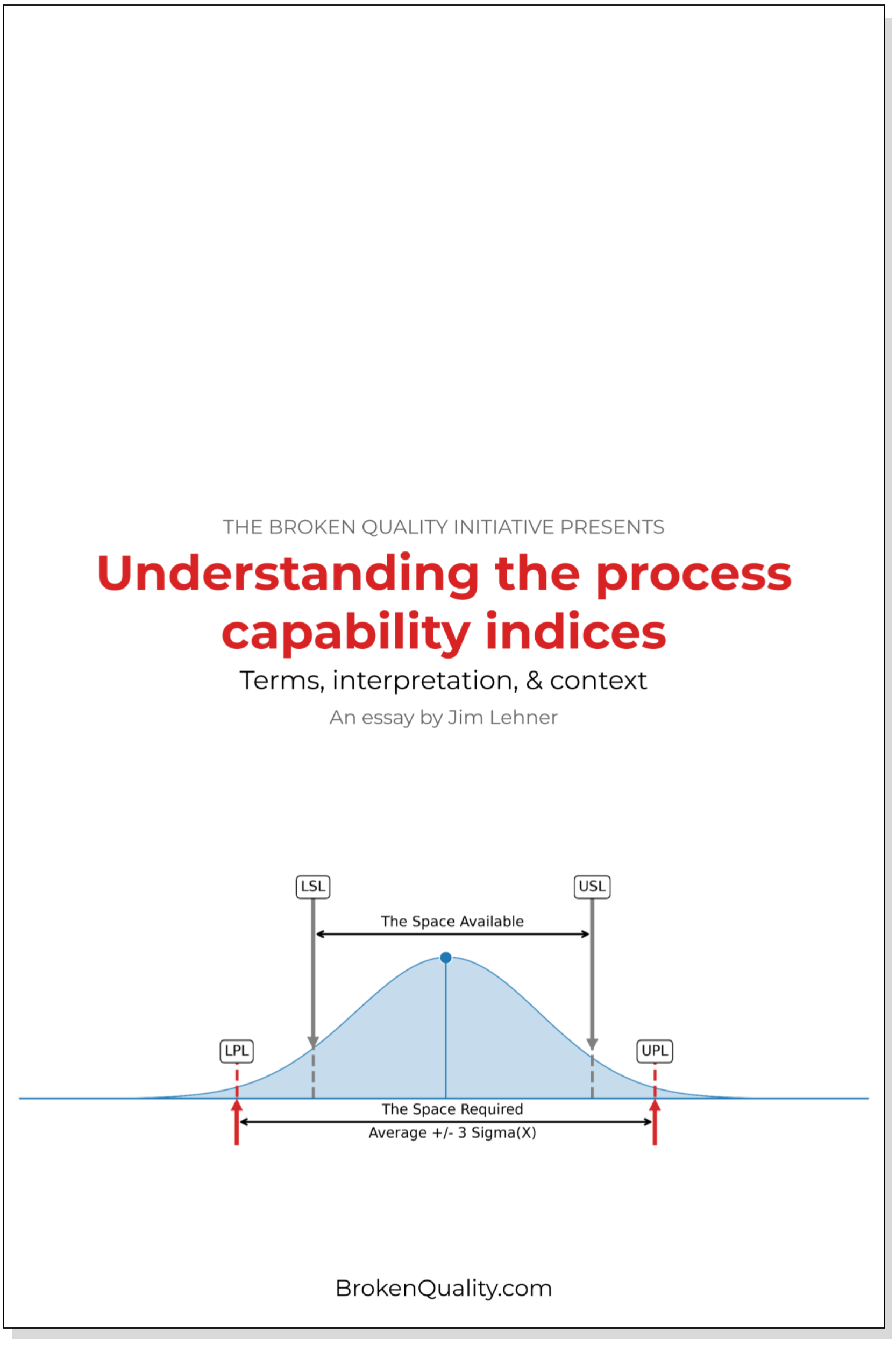
The tolerance defines the acceptable range within which performance or quality characteristics may vary, thereby defining the space available. To calculate the tolerance, subtract the Lower Specification Limit (LSL) from the Upper Specification Limit (USL) using the formula:

Measurements of parts, assemblies, and products that fall inside the specification limits (tolerance) are conforming, while those that fall outside are nonconforming. Thus, the tolerance defines the voice of the customer. It defines what a customer is willing (and not willing) to pay for.
Distance to nearer specification limit, DNS
The distance to the nearer specification, DNS, is the distance from the mean to the nearer specification limit. It serves as a measure of how centered a process is within the tolerance. When the mean is centered at the target, the distance from the mean to each specification limit will be similar (converge). When the mean is biased toward one of the specification limits, the distance from the mean to each specification limit will diverge.
To calculate the DNS, subtract the Lower Specification Limit (LSL) from the mean and subtract the mean from the Upper Specification Limit (USL). The DNS is the smaller of these two values. In practice, calculation of the DNS is achieved using a MIN() function. This function returns the smaller of its two arguments. The formula for the DNS is written as:

When the mean falls inside the specification limits the values returned by the MIN() function will be positive. When the mean is less than the LSL, the (Mean - LSL) term of the MIN() function will be negative. When the mean is greater than the USL, the (USL - Mean) term will be negative.
The DNS will always be less than or equal to one-half of the tolerance. Thus, the relationship between the tolerance and the DNS is written as:

Rewriting this equation in terms of the tolerance yields the formula:

Hence, the DNS quantity, which defines the numerators of the centered capability ratio and the centered performance ratio, reflects how the tolerance bounds the distance from the mean to the nearer specification limit.
Sigma(X)
Sigma(X) is a generic placeholder for one of several within-subgroup measures of dispersion that changes with respect to subgroup size. When a dataset is composed of logically comparable individual values, Sigma(X) is calculated by dividing the average moving range by the bias correction factor, d2 = 1.128.

Readers that are familiar with process behavior charts will recognize the Sigma(X) quantity from Walter Shewhart’s generic formula for calculating process limits, Average ± 3ᐧSigma(X). For process limits to be robust and capable of detecting assignable causes of exceptional variation, a measure of dispersion that is capable of detecting process behavior that is nonhomogeneous is required. The Sigma(X) term uses “the moving ranges to characterize the short-term, point-to-point variation” making it capable of this task.
The quantity 6ᐧSigma(X) that defines the denominators of the capability ratio and the centered capability ratio represents the full span of the three-sigma distance used to calculate process limits. It represents the generic space required by a process (process spread) to operate at its full potential..
If you are unfamiliar with the average moving range, visit BrokenQuality.com/how-to-build-an-xmr-chart to learn more.
Standard deviation
The global standard deviation, s, is the measure of dispersion taught in every introductory statistics course. By way of its calculation, it assumes that a dataset “can be logically considered to be one large homogeneous collection of values, all obtained from the same underlying and unchanging process” (Wheeler, Making Sense of Data, 162). Thus, when a process is operated predictably, the standard deviation summarizes the space used by the process in the past. When a process is operated unpredictably, the standard deviation tends to be inflated. In these instances, it still describes the space used by a process in the past but this description provides no insight into whether or not the process is being operated predictably.

The indices in practice
With an understanding of the terms that compose the process capability indices in hand, the next step is to put them to practice. Enter your email below to download Understanding the Process Capability Indices. This essay puts your new found understanding of the terms to practice. It discusses how the indices are calculated and what their calculation indicates about a process. It also explores how process behavior charts and capability histograms provide the additional context that is necessary to take actions that reduce costs and improve quality.
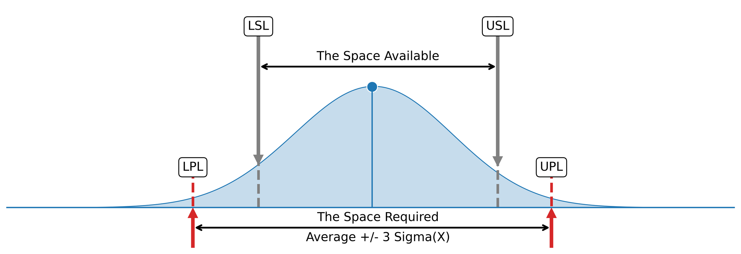
Figure 4. Cp is the space available (defined by the specification limits) divided by the space required (defined by the process limits).
The reader is also encouraged to explore the work of the statistician and quality control expert Donald J. Wheeler at spcress.com. Dr. Wheeler’s work is the foundation of the above discussion and the details outlined in Understanding the Process Capability Indices.