

Sigma(X)
Sigma(X) is a within-subgroup measure of dispersion that changes with respect to subgroup size. It is used in Walter Shewhart’s generic formula for calculating process limits—Average ± 3ᐧSigma(X)—and is also used when calculating the capability ratio (Cp)—Tolerance/6ᐧSigma(X)—and the centered capability ratio (Cpk)—DNS/3ᐧSigma(X). With regard to the capability indices, Sigma(X) is often indicated with the term σ_within (read sigma within). Here, “within” refers to Sigma(X) being a within-subgroup measure of dispersion.
The formula for Sigma(X) can be written using either the average range or the median range, as follows:

Here, R (read R-bar) is the average range of the subgroups of size n and R (read R-tilde) is the median range of the subgroups of size n. d2 and d4 are bias correction factors with values that change with respect to subgroup size. The bias correction factors convert the average range and median range into the appropriate measure of dispersion based on the size of the rational subgroup.
When a dataset is composed of logically comparable individual values, the subgroup size is n = 2, giving the bias correction factors of d2 = 1.128 and d4 = 0.954. In these instances, the average range (R) is represented by the average moving range (mR), or alternatively by the median moving range (mR). Accordingly, the formula for Sigma(X) is written as:

When a dataset is not composed of logically comparable individual values, i.e., it consists of rational subgroups where n > 2, the bias correction factors are determined using Table 1. A CSV version of this table can be found here.
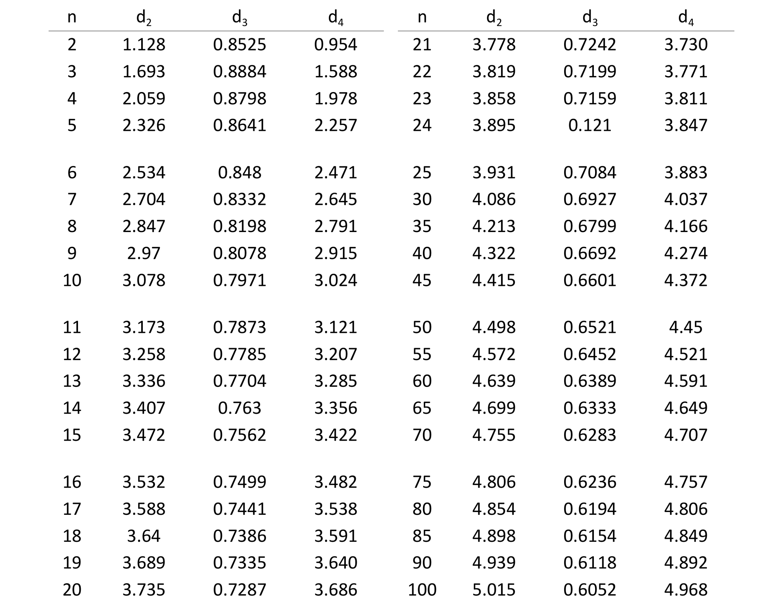
Table 1. Bias correction factors based on subgroup size.
Sigma(X) in practice
Since most individuals that are familiar with process behavior charts rely on software to calculate process limits, it is widely assumed that they are calculated using the generic formula Average ± 3ᐧSigma (or Average ± 3ᐧσ). In these instances, the unaware assume that Sigma is the standard deviation statistic (s), not the within-subgroup measure of dispersion, Sigma(X). While no one can be faulted for not knowing the difference, one can be faulted for continuing to calculate process limits the wrong way.
By way of its calculation, the standard deviation assumes that “the data can be logically considered to be one large homogeneous collection of values, all obtained from the same underlying and unchanging process” (Wheeler, Making Sense of Data, 162). This assumption sits at odds with the intent of the process behavior chart, which “examines a collection of values to see if they might have come from one underlying and unchanging process, or if they show evidence of process changes” (Wheeler, Making Sense of Data, 161).
This mismatch in intent renders the standard deviation ineffective for the calculation of process limits, especially for a dataset that is produced by a process that exhibits unpredictable (nonhomogeneous) behavior. Process limits calculated using the standard deviation will be wider than those obtained using Sigma(X). These wider limits reduce the sensitivity of the process behavior chart and can result in misleading or altogether wrong characterizations of the underlying causal system.
As an example, take the 20 run-out values for hydraulic cylinders in millionths of an inch shown in Table 2.

Table 2. Hydraulic cylinder runout in millionths of an inch.
When process limits are calculated using the formula Average ± 3ᐧSigma(X), where 3ᐧSigma(X) takes the form 2.660ᐧmR, the Upper Process Limit (UPL) is 181.0 and the Lower Process Limit (LPL) is 8.22. This is shown on the left side of Figure 1. Here, one value is greater than the UPL indicating that both common causes of routine variation and assignable causes of exceptional variation have influenced process behavior. Subsequently, the underlying causal system is characterized as unpredictable.
When the process limits for the same data are calculated using the formula Average ± 3ᐧs, where 3ᐧs is three-times the standard deviation, the UPL is 194.1 and the LPL is 0. This is shown on the left side of Figure 1. Here, all of the values fall inside the process limit indicating that only common causes of routine variation influence process behavior. Subsequently, the underlying causal system is characterized as predictable.
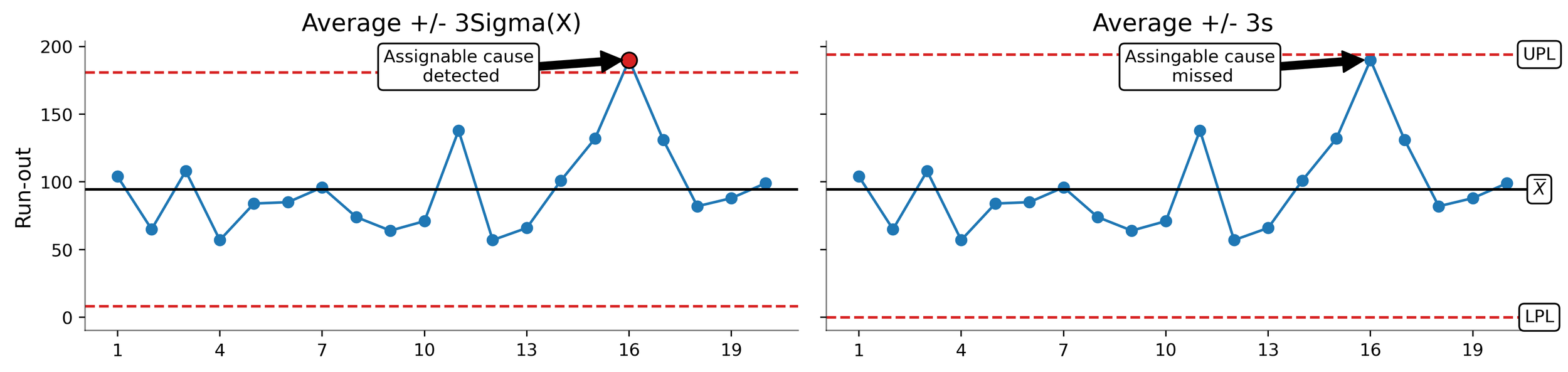
Figure 1. Process limits for hydraulic cylinder runout (in millionths of an inch) calculated using 3ᐧSigma(X) (left) and 3ᐧs (right).
Understanding how process limits are calculated matters. It can be the difference between knowing when it is economical to take action to improve a process and when it is economical to leave a process alone. However, this is only possible when process limits are calculated using the within-subgroup measure of dispersion, Sigma(X).